A working notebook of research ideas, methods I am learning, and
curiosities beyond pavement engineering. Some are developed;
others are questions worth returning to.
Browse the Notebook
Follow a line of thought.
Choose a theme to gather related notes. Some ideas belong to more
than one intellectual thread.
Notebook Threads
Six paths
Showing all notes.
Works in Progress
Two Questions in Motion
Two active lines of inquiry, connected by one concern: turning
material and system response into evidence that supports better
infrastructure decisions.
01Primary focus
Road Infrastructure Resilience
Research question
How can the capacity of road infrastructure to endure,
adapt, and recover be quantified in a meaningful and
decision-useful way?
Quantification
Recovery
Decision support
02Active development
Reflective-Crack Propagation
Research question
How do interlayers alter crack bifurcation, arrest, and
lateral spreading in asphalt mixtures under monotonic
loading?
Bifurcation
Crack arrest
Lateral spreading
A Technical Note
Ways of Reading Asphalt Binder
One material, nine analytical lenses. Start with the question, then choose the evidence.
01
Composition
What is in the binder?
SARA Fractionation
Iatroscan
Four chemical fractions
Saturates, aromatics, resins and asphaltenes reveal the binder's compositional balance.
How to read it
Separation by solubility and polarity yields fractions used to calculate a colloidal index. This helps assess stability and compatibility, but is not a stand-alone prediction of phase separation or brittleness.
CHNS
Elemental analysis
The elemental profile
Carbon, hydrogen, nitrogen and sulfur, measured as mass fractions.
How to read it
A small sample is combusted for analysis. Carbon-to-hydrogen ratios offer clues to aromaticity; sulfur can support comparisons between sources, but cannot identify a crude-oil origin on its own.
XRF
X-ray fluorescence
Trace-element fingerprints
Characteristic X-ray signals reveal elements that bulk composition can miss.
How to read it
Secondary X-rays identify elements such as zinc, copper and molybdenum. Their patterns can help screen for recycled engine-oil bottoms or other additives; attribution needs calibration and corroborating evidence.
02
Molecular fingerprints
How are the molecules changing?
FTIR
Fourier transform infrared spectroscopy
Oxidation fingerprints
Infrared absorption identifies functional groups and tracks chemical aging.
How to read it
Carbonyl and sulfoxide bands are commonly used to form oxidation indices. Compare spectra consistently to assess changes associated with heat and oxygen exposure.
GPC / SEC
Gel permeation / size-exclusion chromatography
Molecular-size distribution
Size-based separation exposes shifts toward larger or smaller molecular species.
How to read it
Elution profiles can track aging-related large-molecular-size fractions and polymer contributions, including SBS. Apparent molecular weights depend on the solvent and calibration.
NMR
Nuclear magnetic resonance
Chemical environments
Hydrogen or carbon signals distinguish aromatic and aliphatic environments.
How to read it
Nuclei respond to a magnetic field according to their local environment. Spectral regions reveal structural features beyond FTIR, rather than a complete map of every molecule in the binder.
03
Transitions & microstructure
What changes with heat and blending?
DSC
Differential scanning calorimetry
Thermal transitions
Heat flow reveals the glass transition and wax-related melting or crystallization.
How to read it
Heating and cooling reveal changes in heat capacity and thermal events. Glass-transition temperature \(T_g\) informs low-temperature behavior; wax estimates require a suitable enthalpy reference.
AFM
Atomic force microscopy
A nanoscale surface map
A scanning probe resolves topography and local surface heterogeneity.
How to read it
Features such as bee structures depend on composition, thermal history and preparation. They are not direct maps of wax or asphaltenes; adhesion interpretation requires complementary measurements.
Fluorescence Microscopy
UV- or blue-light-excited imaging
Polymer dispersion
Optical contrast makes polymer-rich domains and uneven blending visible.
How to read it
Fluorescence contrast can reveal swollen polymer-rich phases, their distribution and agglomeration. Brightness depends on the binder, modifier and illumination, not simply polymer present versus absent.
A Coupled-Materials Note
Chemistry Is Part of the Load Path
Chemical history becomes mechanical consequence.
State ↔ Response
Asphalt is not a mechanically active material with chemistry
sitting quietly in the background. Oxidation, moisture,
composition, and modification alter the molecular state that
rheology and mixture mechanics are attempting to represent.
01Chemical state
oxidation · moisture · composition
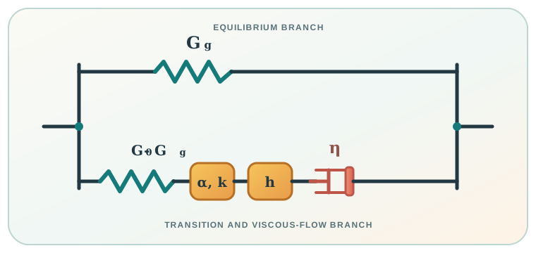
The name 2S2P1D is almost a mechanical inventory: two springs,
two parabolic elements, and one dashpot. Together they describe
the linear viscoelastic response of asphalt binders and mixtures
from the glassy limit, through the broad transition region, to
viscous flow at long loading times.
Elastic limits, distributed transition, and terminal viscous
flow represented in one analogue.
01Glassy bound
\(G_0\) anchors the high-frequency or low-temperature limit.
02Distributed transition
\(k\), \(h\), and \(\alpha\) shape the broad viscoelastic passage.
03Long-time response
\(G_g\), \(\beta\), and \(\eta\) govern the equilibrium and viscous scales.
COMPLEX SHEAR FORMFrequency and temperature meet in \(z=i\omega\tau(T)\).
What I find appealing is its economy: five idealised elements
produce one continuous map of stiffness and phase across loading
rate and temperature. Yet an excellent fit is not, by itself, a
unique molecular explanation; parameter stability, experimental
range, and thermorheological simplicity still have to be tested.
The model was introduced for bituminous binders and mixtures by
Olard and Di Benedetto.
A Rheological Fingerprint
The Cole–Cole Plane: Two Moduli, One Binder
Storage and loss traced together.
G'' versus G'
A Cole–Cole diagram plots the loss modulus (G'') against the
storage modulus (G'). Each DSR observation becomes a point in
the complex-modulus plane; changing temperature or frequency
traces a path that serves as a compact viscoelastic fingerprint
of the asphalt binder.
The trajectory is illustrative: its position and shape should
be compared across binders or conditions, not treated as a
standalone performance threshold.
(G') records stored elastic energy; (G'') records viscous dissipation.
02Path
Temperature and loading rate order the observations along the trajectory.
03Change
Shifts or altered curvature can reveal a changed relaxation architecture.
I like the diagram because it refuses to split elasticity and
viscosity into separate stories. Aging, foaming, or modification
may move or reshape the path, but the interpretation is strongest
when read alongside master curves, Black diagrams, and model
parameters rather than in isolation.
A Black diagram removes temperature and loading frequency from
the visible axes and places every DSR observation in a plane
defined by phase angle \(\delta\) and complex shear modulus
\(|G^*|\). The resulting path becomes a compact rheological
fingerprint: stiffness, viscoelastic balance, and departures
from simple time-temperature equivalence can be read together.
Every point represents a DSR measurement; temperature and
frequency are encoded along the path rather than shown as axes.
Up and left is stiffer and more elastic; down and right is softer and more viscous.
02Read shape
A smooth collapse supports simple shifting; shoulders, loops, or scatter invite investigation.
03Read movement
Ageing and modification can relocate or reshape the path, revealing a changed response architecture.
What appeals to me is the economy of the representation. Two
familiar rheological quantities turn many temperatures and
frequencies into one visual argument. The diagram does not replace
constitutive modelling or performance testing, but it can reveal
where the binder behaves simply, where its structure intervenes,
and where the data themselves deserve another look.
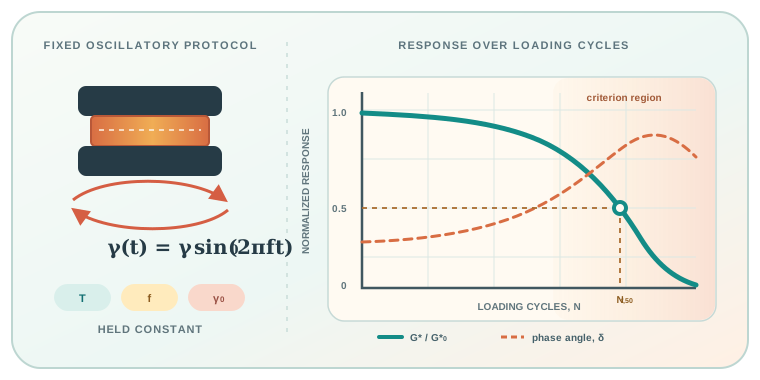
A time sweep asks a deliberately simple question: what happens
when an asphalt binder is sheared again and again under the same
nominal conditions? In a dynamic shear rheometer, temperature,
frequency, and loading amplitude are held fixed while the
material response is recorded cycle by cycle.
The familiar 50% modulus point is a useful convention, not an
automatic proof that every preceding change was fatigue damage.
01Hold fixed
Temperature \(T\), frequency \(f\), and strain \(\gamma_0\) or stress amplitude.
02Track
Complex modulus \(G^*\), phase angle \(\delta\), and dissipated energy through cycle \(N\).
03Interpret
Rate of change, failure criterion, strain sensitivity, and any recovery after rest.
\[
\begin{aligned}
\gamma(t)&=\gamma_0\sin(2\pi f t),\\
W_d(N)&=\pi\gamma_0^2G^*(N)\sin\delta(N).
\end{aligned}
\]
Under strain-controlled loading, a larger imposed amplitude
generally drives a faster reduction in \(G^*\) and a shorter
apparent fatigue life. A common definition, \(N_{f,50}\), is
the cycle at which \(G^*\) reaches 50% of its initial value.
Other interpretations use peaks in phase angle or stiffness
multiplied by cycle count, dissipated-energy ratios, or
continuum-damage concepts.
The caution is as important as the curve. Self-heating,
thixotropy, nonlinear response, radial flow, and edge fracture
can reduce the measured modulus alongside genuine damage. A
binder time sweep is therefore a rich comparative rheological
probe, but not a direct translation of pavement fatigue life.
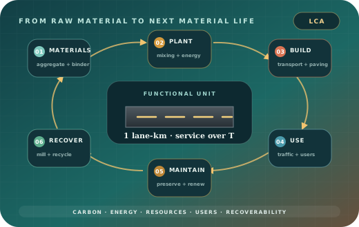
Sustainability in flexible pavement engineering cannot be judged
from the asphalt mixture alone. A pavement begins with aggregate
extraction and binder production, remains environmentally active
through construction and use, and continues beyond milling into
recycling, recovery, or disposal.
The system boundary follows the pavement from raw material to
service, intervention, and its next material life.
Materials, transport, construction, use, maintenance, rehabilitation, and end of life all belong inside the ledger.
02Compare equal service
A lower plant impact is not an improvement if it produces earlier intervention or poorer performance elsewhere.
03Test circular claims
RAP, warm mix, durable binders, and preservation matter through their total effects on demand, energy, service life, users, and recovery.
LCA is not a label of greenness. It is a transparent accounting
system for asking whether a pavement delivers more service with
less environmental burden.
Machine learning becomes much clearer when it is framed as a
measurable change rather than as computational mystique. A system
is given experience (E), asked to perform a task (T), and
judged by a performance measure (P). Learning has occurred only
if further experience improves that measured performance.
Two complementary views: learning must improve something we can
measure, while probabilistic modelling keeps uncertainty visible.
EExperience
The observations, examples, feedback, or interactions from which the system can change.
TTask
The operation to be learned: classification, prediction, ranking, control, or another defined objective.
PPerformance
The criterion that makes improvement testable rather than impressionistic.
Predictions, parameters, and unobserved states are rarely
known exactly. Representing them with probability
distributions records both what the model expects and how
strongly the available evidence supports that expectation.
Data (D) updates uncertainty about ( heta); the resulting
posterior can then support a decision under uncertainty.
I like this formulation because it imposes discipline before
architecture: define the task, choose an honest measure, state
what constitutes experience, and preserve uncertainty in the
conclusion. Probability then becomes a common language linking
machine learning with statistics, engineering, control, and
decision science.
In supervised learning, the experience is a collection of
examples for which the desired output is already known. The task
is to learn a mapping from an input
x ∈ 𝒳 to an
output y ∈ 𝒴,
then use that mapping when a new input
arrives without its answer attached.
The Iris example turns four measurements into one of three
species labels; the principle extends to both classification
and regression.
THE DATA
\[
\begin{aligned}
\mathcal D&=\{(x_n,y_n)\}_{n=1}^{N},\\
x_n&\in\mathbb R^D,\qquad y_n\in\mathcal Y.
\end{aligned}
\]
Turn each observation into informative and consistently measured features.
02Label
Attach the class, value, or response that the model is expected to predict.
03Fit
Choose parameters that reduce a task-appropriate loss on the training examples.
04Generalize
Judge the learned rule on untouched examples, not by its memory of the training set.
I like supervised learning because its contract is unusually
explicit: specify what is observed, state what must be predicted,
define the penalty for being wrong, and reserve evidence that can
challenge the fitted model. The sophistication of the algorithm
never removes the need for trustworthy labels and an honest test.
Empirical Risk Minimization: Turning Error into an Objective
Define the cost. Average it. Minimize it.
min R̂
A model cannot improve until “wrong” has a numerical meaning. A
loss function assigns a cost to each prediction; empirical risk
is the average of those costs over the observed training set.
Empirical risk minimization chooses the model parameters that
make this average as small as possible.
The loss function creates the landscape; optimization searches
that landscape for a parameter setting with lower average cost.
Useful for misclassification rate when all wrong labels are treated equally.
THE CONSEQUENCE MATTERSCost-sensitive loss
\[\ell_C(y,\widehat y)=C_{y,\widehat y}.\]
Appropriate when one kind of mistake is more damaging than another.
01Predict
Apply fθ to every training input.
02Penalize
Translate each discrepancy into a loss.
03Average
Summarize the sample as R̂N(θ).
04Optimize
Search for parameters with lower empirical risk.
I find ERM appealing because it exposes every modelling choice:
the examples define the evidence, the loss defines what matters,
and the optimizer follows the geometry produced by those two
decisions. Before asking which algorithm is best, one should ask
whether the chosen loss represents the real consequence of error.
First count the mistakes. Then ask what each mistake costs.
loss / N
Misclassification rate treats every incorrect label identically:
a correct prediction contributes zero and an incorrect prediction
contributes one. Empirical risk keeps the same averaging structure
but replaces this fixed penalty with a loss function capable of
representing severity, asymmetry, or scientific consequence.
The denominator does not change. What changes is the information
carried by each term in the numerator.
Compare each predicted label with the corresponding truth.
02Value
Use a loss function to encode the consequence of the discrepancy.
03Average
Combine the individual losses into one sample-level measure.
This small mathematical substitution changes the question from
“How often is the model wrong?” to
“How costly are its errors on the evidence we observed?”
The second question is often closer to the decision we actually
need to make.
Reward probability assigned to what actually occurred.
MLE
For a probabilistic model, a natural loss is the negative log of
the probability assigned to the observed outcome. A confident,
correct prediction receives a small penalty; assigning little
probability to the truth receives a large one.
PROBABILITY OF THE OBSERVED TRUTHThe negative logarithm turns confidence into cost.
Negation reverses the direction; the logarithm turns a product into a sum without changing its maximizer.
Thus, empirical-risk minimization with negative log loss is not a
separate fitting principle: under the probabilistic model, it is
maximum-likelihood estimation written in the language of loss.
Training performance is evidence of fit, not proof of generalization.
Δgen
A sufficiently flexible model can drive training loss toward zero
by capturing both structure and accidental detail. Generalization
asks a harder question: does the fitted rule remain accurate on
observations that did not participate in fitting or model
selection?
The lowest training loss lies at the far right; the preferred
model lies near the minimum validation loss, before complexity
begins to fit sample-specific noise.
Estimate parameters and gradients using the training observations.
02Select on validation data
Choose capacity, hyperparameters, and stopping rules without consulting the test set.
03Report on test data
Estimate final out-of-sample performance only after model choices are fixed.
The point of learning is not to explain the examples already in
hand as intricately as possible. It is to discover enough stable
structure that the rule survives contact with the next example.
A model earns trust by surviving a purpose, not by becoming reality.
model ≠ world
“
All models are wrong, but some models are useful.
George E. P. Box
assumecompareuserevise
A model is a deliberate compression of the world. It ignores
detail so that a pattern can be calculated, communicated, or used
to decide. Its omissions are not automatically defects; they
become defects when they erase what matters for the question at
hand.
A SMALL FORMALISMAdequacy is conditional on task, domain, and tolerance.
Name the prediction, explanation, comparison, or decision the model must support.
02Useful where?
State the population, loading regime, scale, and conditions that define its domain.
03Wrong in which way?
Identify the errors that are tolerable and those that would invalidate the intended use.
01 Simplify→02 Confront→03 Use→04 Revise
The sentence is not an argument against modelling. It is an
argument for intellectual humility: make assumptions visible,
test consequences against evidence, respect the boundary of the
model’s domain, and revise it when reality refuses to cooperate.
A Probabilistic Note
Uncertainty: Knowing What the Model Does Not Know
A probability is a degree of belief, not a guarantee.
p(y | x)
Exact prediction is often impossible. Sometimes the model lacks
knowledge; sometimes the observation itself is noisy or compatible
with several outcomes. A responsible model represents this
ambiguity as a distribution over possible outputs rather than
concealing it behind a single confident label.
One prediction can distribute belief across several outcomes;
the reason for that spread determines what should happen next.
FROM SCORES TO PROBABILITIESSoftmax normalizes the class evidence.
EPISTEMIC · MODEL UNCERTAINTYUncertainty from limited knowledge.
Sparse coverage, unfamiliar inputs, uncertain parameters, or
an inadequate model can make several explanations plausible.
Better-targeted data or a better model may reduce it.
Ask: what evidence would change the model?
ALEATORIC · DATA UNCERTAINTYUncertainty within the observation process.
Measurement noise, class overlap, and inherent stochasticity
can leave different outcomes plausible even with a well-learned
model. Repeating the same information does not remove it.
Ask: what ambiguity remains at fixed information?
01Act
When uncertainty and consequences are both acceptably low.
02Investigate
Gather a test, measurement, or expert review when information may help.
03Abstain
Defer the decision when uncertainty and the cost of error are both high.
What matters is not merely whether the model is uncertain, but
why. Epistemic uncertainty invites learning; aleatoric uncertainty
invites caution; decision theory asks what each possible mistake
would cost. A model that can express doubt is often more useful
than one that is confidently wrong.
Convolutional neural networks: learning structure from images.
I am studying CNNs because I expect to use image-based pattern
recognition in my current work. Their appeal lies in a disciplined
progression: learn locally, reuse what is learned, and assemble
simple features into increasingly meaningful representations.
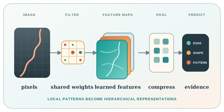
A conceptual CNN pipeline: local filters transform pixels
into a hierarchy of learned evidence.
01Local perception
Small kernels inspect neighborhoods rather than treating every pixel independently.
02Shared weights
The same filter searches across the image, reducing parameters and preserving spatial logic.
03Feature hierarchy
Edges and textures can combine into shapes, objects, and task-specific patterns.
CNNs are among the most influential architectures in modern
machine learning because they make image structure part of the
model itself. Convolution, nonlinear activation, and pooling
provide a relatively clear entry point into how neural networks
turn visual information into a prediction.
My aim is to understand this architecture from the foundations
upward rather than treat it as a black box. That means asking
not only whether a network is accurate, but what evidence it
learned, whether the dataset permits that claim, and whether the
result remains stable beyond the images used for training.
Starting point
A gentle introduction for readers who want an entry into CNNs is
arXiv:1511.08458.
An Intellectual North Star
Grigori Perelman
Depth without spectacle.
RIGOR
Grigori Perelman remains very much on my mind. His
intellectual courage, depth, and refusal of spectacle form a
rare model of what it means to pursue an idea with absolute
seriousness and without compromise.
A mathematician whose work and choices resist spectacle.
01Depth
Stay with the problem beyond its fashionable surface.
02Independence
Let the work, rather than spectacle, establish its seriousness.
03Integrity
Hold intellectual standards without bargaining them away.
Ricci flow lets a metric evolve in response to curvature.
Perelman's work made this evolution part of a profound route
through topology, singularity, and geometric structure.
curvatureentropysurgerytopology
What stays with me is the union of imagination and discipline:
an immense problem approached without theatricality, and a life
that makes intellectual seriousness feel almost physical.
Current Curiosity
Rayleigh Distribution and the Stress-Strain Curve
A statistical lens for nonnegative response features.
\(R\geq0\)
I want to understand whether the Rayleigh distribution can offer
a useful language for selected features extracted from families
of stress–strain responses. The attraction lies in connecting a
disciplined probability model to visible mechanical variability,
without confusing a distribution with a constitutive law.
A possible workflow: define a physically meaningful nonnegative
feature, observe it across specimens, then test whether the
Rayleigh assumptions survive the data.
THE GEOMETRIC ORIGINThe magnitude of two independent Gaussian components
The density begins at zero, rises to a mode at \(r=\sigma\), and then decays.
02Scale
\(\sigma\) controls both the characteristic magnitude and the spread.
03Mechanical question
Could peak stress, strain at a feature, or a response amplitude behave like \(R\)?
What interests me is the bridge itself: moving from the geometry
of a probability distribution to a falsifiable question about
material response, while keeping statistical description and
mechanical interpretation rigorously distinct.
A Thought
Rheology, Theology, and the Deborah Number
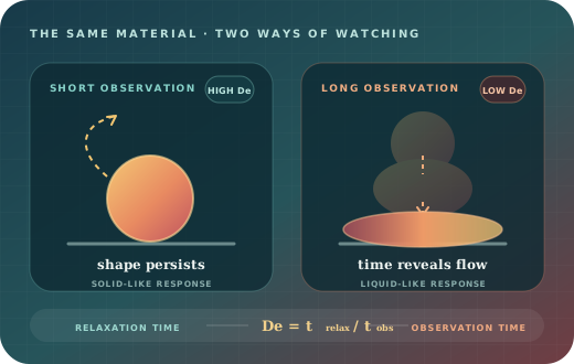
De
The Deborah number asks a deceptively simple question: how long
does a material need to relax compared with how long we choose to
observe it? What appears permanent may simply be changing more
slowly than our experiment allows us to see.
The material has not changed identity; only the competition
between its relaxation time and our observation time has changed.
Observation is fast relative to relaxation, so the response appears solid-like.
LOW \(De\)Shape yields to time
Observation is long relative to relaxation, so flow becomes visible.
This is where rheology meets a theological image. The biblical
line often paraphrased as “the mountains flowed before the Lord”
gains a material meaning: wait long enough and even mountains
move. The Deborah number is therefore more than a ratio to me; it
is a reminder that permanence is often a matter of timescale.
Howard A. Barnes and his colleagues discuss this beautifully in
An Introduction to Rheology, which is a book I love and keep returning to.
A Mathematical Aside
Erdős Number
Collaboration measured as distance.
distance
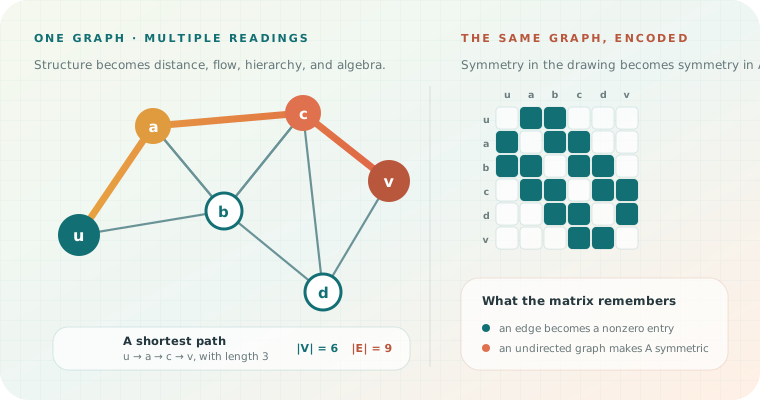
3
The Erdős number turns collaboration into something almost
topological. It is playful, but it also says something serious
about how mathematical work travels through people, papers, and
shared intellectual lineages.
A path of length three means three coauthorship links connect
the author \(v\) to Paul Erdős.
In that sense, a whimsical academic fact becomes a clean
expression of connectedness inside a scholarly network. It also
reminds me why graph theory fascinates me: intellectual life can
be read as relation, path, reachability, and structure.
In that spirit,
Network Science
by Albert-László Barabási is a wonderful read.
A Mathematical Aside
Poisson Distribution
Order hidden inside scattered events.
λ
The Poisson distribution has an austere elegance: it counts how
often an event occurs when arrivals are independent and governed
by a steady average rate. One parameter is enough to give
apparently scattered events a disciplined shape.
A continuous interval, a discrete count: here \(X=4\) is one
possible realization when \(\lambda=4\).
This equality of mean and variance is the signature I find most
memorable. The model says something surprisingly economical:
randomness can have structure without losing its randomness.
A Mathematical Infatuation
Graph Theory
The geometry of connection.
G = (V, E)
I am quite genuinely infatuated with graph theory. There is
something deeply satisfying about the way it reduces structure,
relation, and complexity to a language that is both austere and
expansive. A few vertices and edges can contain distance, flow,
centrality, cycles, spanning trees, and entire geometries of
interaction.
One object, several readings: a drawing reveals relation, a path
reveals distance, and a matrix makes the structure computable.
01
The object
A finite vertex set \(V\) and a set \(E\) of unordered pairs define a simple undirected graph.
What I love here is not only the formalism, though the formalism
is beautiful, but its persistence: collaboration networks,
infrastructure systems, transport, diffusion, reliability, and
the movement of ideas all become legible through relations.
Graph theory feels less like a chapter of mathematics and more
like a durable way of seeing.
Topology by Gluing
A Square That Remembers Two Circles
The torus is periodicity made visible.
T²
A torus is the mathematical surface of a doughnut, but its most
revealing construction begins with a square. Identify the left
edge with the right edge and the square becomes a cylinder;
identify the cylinder's two circular ends and it closes into a
torus.
Gluing does not erase direction: it turns each independent
translation into a closed loop.
One Direction
A line closes into a circle
Positions separated by an integer are treated as the same point.
The square is a fundamental domain: copies tile
the infinite plane, while edge identification records how one
copy wraps back onto itself.
The Same Idea, Two Complex Dimensions
If \(\Lambda\subset\mathbb C^2\) is a rank-four lattice, then
\(\mathbb C^2/\Lambda\) is a complex two-torus—four real
dimensions built by making four independent directions periodic.
The doughnut is only the first picture of a much larger idea.
When Abstraction Finds the World
The Unreasonable Effectiveness of Mathematics
Why does an invented language fit nature so precisely?
Wigner · 1960
Wigner's puzzle is not simply that equations can describe
measurements. It is that structures cultivated in relative
independence from experience—complex numbers, operators, and
abstract spaces—later become the precise language of phenomena
they were not designed to explain.
Abstract structureπ · i · ∂ · H
logic, symmetry, and form
Φ→
interpret
Observed worldorbit · spectrum · field
measurement and prediction
Ideas formed in one mathematical setting become useful in another physical domain.
02Unreasonable precision
The agreement can reach far beyond the observations that first suggested the theory.
03Predictive reach
The formalism reveals consequences that were not explicitly placed in its starting data.
What stays with me is Wigner's restraint. Mathematical success is
not proof that a model is reality, and every law remains bounded by
its domain. It is a recurring scientific gift: powerful enough to
use, mysterious enough to keep questioning.
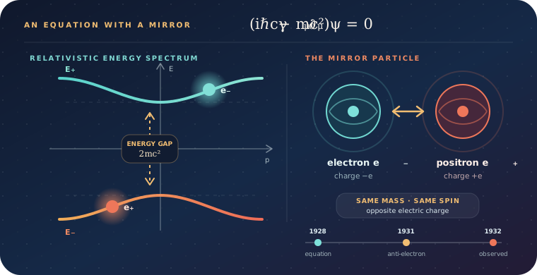
When mathematical symmetry enlarged the material world.
e− ↔ e+
Dirac trusted an equation far enough to let it describe matter
that no one had yet seen. In bringing quantum mechanics into
accord with special relativity, he obtained not only a theory of
the electron, but a mathematical mirror that the known inventory
of nature could not yet fill.
The relativistic spectrum carries two signs; physical
interpretation turns the apparent surplus into matter–antimatter symmetry.
A first-order wave equation had to respect both quantum mechanics and special relativity while accounting naturally for electron spin.
02
The mathematical surplus
The relativistic energy relation admitted positive and negative branches. The unwanted solutions could not simply be wished away.
03
Nature answers
The anti-electron would have the electron’s mass and spin but the opposite charge. Anderson’s positron supplied the experimental answer.
In that sense, Dirac conceived half of the material universe in
his mind before experiment revealed it. It remains one of the
loveliest examples of disciplined imagination: mathematics did
not decorate an observation; it insisted that nature was larger,
stranger, and more symmetrical than observation had yet shown.
I keep returning to reading not merely as an academic obligation,
but as a practice that enlarges inner life, sharpens judgment, and
develops seriousness of thought. Information may be collected
quickly; intellectual depth usually has to be read into being.
Film and research may ask different questions, but both depend
on sustained attention before expression.
01Enlarge
Build an inner archive of voices, histories, methods, and unfamiliar ways of seeing.
02Sharpen
Develop the judgment to distinguish an interesting claim from a merely fashionable one.
03Deepen
Stay with a problem long enough for better questions to replace the first easy answers.
Werner Herzog’s repeated insistence to read, read, read
feels demanding and liberating. He says it in the context of
filmmaking, but it applies just as strongly to research, where
depth of thought is often inseparable from depth of reading.
The destination is simple. Preserving the self is not.
NOSTOS
Homer gives us a journey whose endpoint is known almost from the
beginning: Ithaca. The difficulty is not identifying home, but
passing through appetite, pride, grief, delay, and enchantment
without forgetting why one wished to return.
Selected episodes, arranged conceptually rather than
geographically: the route wanders, while the idea of home
remains the hidden coordinate.
01 · WORLD\(G=(V,E)\)
Islands, thresholds, and seas become vertices and passages in a directed graph.
02 · TRAVELLER\(s_t=(x_t,m_t)\)
\(x_t\) is location; \(m_t\in[0,1]\) is memory of home and purpose.
Perhaps that is why the poem remains so alive. Every life has an
Ithaca, but the more interesting variable is what survives in us
while we are trying to reach it.
A Note on the Inner Landscape
The Old Patterns Beneath New Stories
Carl Jung, archetypes, and the work of becoming whole.
Ψ
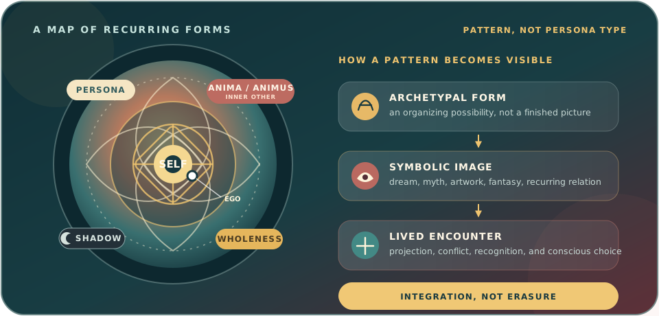
For Jung, an archetype is not a stock character, a personality
label, or an inherited picture. It is a recurring organizing
pattern within the collective unconscious—a form we encounter
indirectly through dreams, myths, art, relationships, and the
symbols a culture gives to difficult human experience.
The archetype is not the image itself. It is the recurring
pattern around which many different images can gather.
Archetypethe organizing pattern
Never encountered in a final, culturally neutral form.
→Symbolthe pattern made imaginable
Historically situated, personal, revisable, and alive.
01
Persona
The social face that helps a person meet the world. Necessary, but dangerous when mistaken for the whole self.
02
Shadow
Qualities and possibilities the conscious ego does not readily own. The shadow is not simply evil; it may also contain neglected vitality.
03
Anima / Animus
Jung's historically gendered language for an inner other. It is most useful today as symbolic polarity, not a rigid identity rule.
04
Self
The organizing symbol of psychic wholeness: larger than the conscious ego, and capable of holding tension without pretending it has vanished.
Archetype ≠ fixed character
one pattern → many symbolic forms
Individuation, then, is not the production of a flawless self.
It is the difficult practice of becoming less divided and less
governed by what remains unexamined—bringing persona, shadow,
inner other, and conscious purpose into a more honest relation.
An Eclipse, A Verdict
Eddington and the Bent Light
1.75
arcsec
Einstein's general theory of relativity made a precise and
audacious prediction: the Sun's gravity should bend passing
starlight, shifting the apparent position of a star near the
solar limb. The eclipse supplied a way to see the otherwise
invisible geometry.
Hide the Sun, photograph the surrounding stars, then compare
their eclipse positions with a reference plate.
Relativity specifies how much starlight grazing the solar limb should bend.
02Reveal
On 29 May 1919, totality made nearby stars photographable from Príncipe and Sobral.
03Compare
Eclipse plates and reference plates turn apparent stellar displacement into a test.
The results announced by Frank Dyson, Eddington, and Andrew
Crommelin were consistent with Einstein's prediction and became
the celebrated first observational confirmation of general
relativity. I find the scene irresistible: an eclipse made the
geometry of spacetime visible, and an idea formed in equations
left a measurable mark upon the sky.
Interstellar makes time dilation emotional before it
makes it mathematical. On Miller's planet, deep within the
gravitational environment of Gargantua, one hour for the landing
party corresponds to seven years far from the black hole.
The observers separate in spacetime, not merely in space; their
clocks reunite carrying different histories.
A simple Schwarzschild clock at radius \(r\) accumulates proper time as
\[
d\tau=dt\sqrt{1-\frac{2GM}{rc^2}}.
\]
02
Motion changes it too
Relative motion contributes the familiar special-relativistic factor
\[
d\tau=dt\sqrt{1-\frac{v^2}{c^2}}.
\]
That is what gives the sequence its force. Cooper does not merely
travel far from home; he returns displaced in time from the people
he loves. Relativity becomes loss measured not in distance, but in
years. There is no universal clock shared by every observer.
Time dilation has a spatial companion. An object has its greatest
length L0 in the frame where it is at rest. An observer who
sees it move at speed v measures a shorter longitudinal length
L, provided the positions of both endpoints are recorded at
the same time in that observer’s frame.
The transverse size is unchanged in the illustration; only the
dimension parallel to the relative velocity contracts.
Measure the endpoints in the object’s rest frame. This is the maximum spatial length assigned to the object.
02
Contracted length L
Measure both moving endpoints simultaneously in the observer’s frame. The result is L0/γ.
0.60cL = 0.800L00.80cL = 0.600L00.99cL ≈ 0.141L0
The lesson is quietly radical: there is no observer-independent
answer to “how long is it?” until the frame and the simultaneity
convention are specified. Space, like time, participates in the
geometry of relative motion.
A Relativistic Thought Experiment
The Twin Who Returned Younger
20 y/12 y
Two twins synchronize their clocks. One remains on Earth; the
other travels to a distant star at high speed, turns around, and
returns. At reunion, less time has elapsed for the traveller.
The clocks are not confused: they have measured two different
paths between the same meetings.
The Earth twin follows one inertial worldline; the travelling
twin changes inertial frames at the turnaround.
During either constant-speed leg, each twin may describe the other clock as running slowly.
THE MISSING DISTINCTION
Only one twin changes frame
The traveller switches from the outbound frame to the inbound frame; the Earth twin does not.
Neither twin owns the universal clock because there is no
universal clock. In relativity, elapsed time belongs to a path
through spacetime, not merely to its starting and ending events.
The Grand Unfinished Question
Hawking and the Unfinished Equation
Can one framework speak for the very large and the very small?
GR + QM → ?
Modern physics rests on two astonishingly successful languages.
General relativity describes gravity as the geometry of spacetime;
quantum theory describes matter and fields through quantized states
and probabilities. Each works beautifully in its own domain. The
difficulty begins where both must speak at once.
Black holes force the two theories into the same room. Hawking
radiation is a profound clue, but not yet the completed union.
A deeper framework should contain gravity and quantum physics without contradiction and recover their successful predictions where each already works.
02 · THE OBSTACLE
Spacetime must become quantum
Quantum fields usually evolve on a spacetime background; relativity says that background is itself dynamical. At extreme scales, that separation fails.
03 · HAWKING'S CLUE
Black holes are laboratories
Hawking showed that quantum fields near a horizon produce thermal radiation, binding gravity, quantum theory, and thermodynamics into one unavoidable puzzle.
What I find moving in Hawking's search is its scale of ambition
joined to intellectual humility. The dream was not merely to find
a shorter equation, but to understand why the universe can be
described coherently from quantum fluctuation to cosmic history.
The unfinished center is not a failure; it is the frontier.
The AI Futures Project's AI 2040: Plan A is not
presented as its authors' most likely forecast. It is a
positive policy scenario: slow the race to superintelligence,
make frontier research inspectable, and preserve human control
long enough to build a credible safety case.
The United States and China agree to a verified slowdown and
declare the frontier compute they control.
2030
Brake the loop
The agreement blocks automated AI research from turning
capability gains into a rapid, self-reinforcing takeoff.
2035
Hold the line
Development pauses near top-human-expert capability, buying
time for alignment, oversight, and institutional learning.
2040
Conditional handoff
Scaling resumes only when the safety case is judged stronger
than the risks of continued delay.
01
Verify the compute
Chip accounting, mutual declarations, audits, inference-only
controls, and secured research clusters make the slowdown
enforceable without relying on trust alone.
02
Open the research
Algorithms, experiments, code, and safety cases become open
to scrutiny, while dangerous model weights and sensitive data
remain protected.
03
Titrate capability
Scale toward the strongest AI that remains confidently
controllable, then slow almost to a halt rather than racing
through an intelligence explosion.
The five pressures Plan A confronts
Loss of control
Concentrated power
Great-power conflict
Labor displacement
Catastrophic misuse
What interests me most is the discipline of scenario scrutiny.
Instead of saying that governance will somehow catch up, the
proposal has to survive dates, incentives, verification limits,
institutional weakness, and the possibility of defection. Whether
or not one accepts Plan A, that is a serious way to think about a
future arriving faster than our institutions can comfortably
reason about it.
Are You Up?
A small numbers game.
There is a hidden number between 1 and 31. You have six attempts.
I'll tell you if the guess should go higher or lower.